The Mathematics of the Electoral College: Anchor States, Power Indices, and Long-Term Lock-In

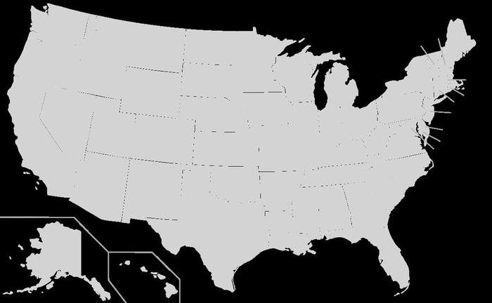
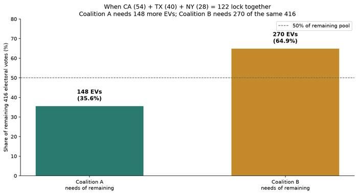
Think of a presidential race as a scoreboard with 538 points. The first side to 270 points wins. California is worth 54 points. Texas is worth 40. New York is worth 28. Add those three together and you get 122 points before anyone else votes. Call the side that holds them Coalition A. Call the other side Coalition B. Coalition A then needs only 148 more points out of the 416 that remain — about one third. Coalition B needs 270 of those same 416 — nearly two thirds. That is a steep climb for Coalition B, and an easier path for Coalition A. The rest of this article is the math behind that gap, and what it means if it lasts.

Those three jurisdictions alone hold 122 electoral votes — 22.7 percent of the College. When they vote together, the remaining contest is a fight over 416, not 538. The coalition that holds the 122-vote anchor needs only 148 more electoral votes to reach 270 — 35.6 percent of what is left. The opposing coalition must take 270 of those same 416 — 64.9 percent of the remainder. That asymmetry is arithmetic, not a political claim.

§ 1How the weights are built

Each state's electoral vote total equals its two senators plus its seats in the House of Representatives. House seats are reapportioned after every decennial census by the Huntington–Hill method of equal proportions, which has been the statutory rule since 1941. The method first gives every state one seat, then assigns the remaining 385 seats by ranking priority values. For a state with population P that already holds n minus 1 seats, the priority for its next seat is P divided by the square root of n times (n minus 1). That geometric-mean divisor is what sets Huntington–Hill apart from older rounding rules, keeping relative representation gaps as small as possible across states of very different sizes.

The Twenty-Third Amendment then gives the District of Columbia three electors, the same floor that the smallest states receive. The result is a hard minimum of three electoral votes for every jurisdiction and a maximum that currently belongs to California at 54. The floor creates a well-known imbalance in people per elector. Using 2020 Census apportionment populations, Wyoming has roughly 193,000 residents per electoral vote. California has roughly 733,000. Texas sits near 730,000. A Wyoming elector therefore represents about one-third as many people as a California or Texas elector. That is the small-state premium baked into the two-senator add-on.

There is a second, subtler effect that cuts the other way. In a weighted voting game, a large bloc is more often pivotal than its raw share of the total suggests — the large-state premium in voting power. The two effects do not cancel; both matter for the probability analysis that follows. Maine and Nebraska can split electors by district; every other state is winner-take-all. For national coalition math, those splits are a small perturbation. The decisive structure remains the 51-jurisdiction game with quota 270.

§ 2The fifteen-plus club

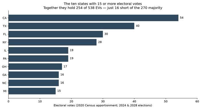
Under the 2020 Census allocation that governs 2024 and 2028, exactly ten jurisdictions hold 15 or more electoral votes: California 54, Texas 40, Florida 30, New York 28, Illinois 19, Pennsylvania 19, Ohio 17, Georgia 16, North Carolina 16, and Michigan 15. Their combined weight is 254 — only 16 short of a majority. Ten jurisdictions out of fifty-one already control nearly the entire quota. A three-vote flip in Wyoming barely moves the path to 270. A forty-vote flip in Texas rearranges it.

§ 3Power indices: Banzhaf and Shapley–Shubik

Raw electoral votes measure weight. They do not measure power. Power, in the formal sense used in cooperative game theory, is the frequency with which a player is critical — the player whose departure turns a winning coalition into a losing one.

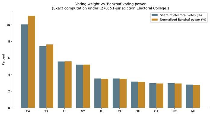
The Banzhaf index counts, for each jurisdiction, how often its votes tip a coalition across the 270 quota. Computed exactly by dynamic programming on the 51 weights, California's absolute Banzhaf probability is about 0.461, and its normalized share is 11.08 percent of total criticality. California's electoral-vote share is only 54 out of 538, or 10.04 percent. The ratio, about 1.10, is the large-state power premium. Texas sits at 7.64 percent of Banzhaf power against a 7.43 percent vote share. New York is essentially proportional at 5.21 percent versus 5.20 percent. The smallest three-vote jurisdictions fall slightly below their vote share.

The Shapley–Shubik index averages criticality over all orderings in which jurisdictions join a coalition. Exact values put California at 10.80 percent, Texas at 7.74 percent, and New York at 5.28 percent. Both indices agree that California's voting power exceeds its vote share. They assume every coalition is equally likely; real elections are correlated. Power indices still measure the structural advantage of weight; correlated models measure how often a given alignment actually wins.

There is also a two-stage version of the same idea, tracing back to L. S. Penrose's square-root law. Inside a winner-take-all state, a single voter's chance of breaking an exact tie scales roughly with one over the square root of the state's population; the state's electoral-vote bloc then carries that tip into the national game. An individual voter's combined Banzhaf power is proportional to the state's absolute Banzhaf score divided by the square root of its population. Under current weights, that ratio for a California voter is about 2.45 times Wyoming's; Texas sits near 2.0, New York near 1.6. Even though Wyoming has far more electors per person, a California voter still has roughly two and a half times as much two-stage tipping power.

§ 4The California–Texas–New York anchor

Fix California, Texas, and New York as a single 122-vote bloc for Coalition A. The reduced game for the remaining 48 jurisdictions has total weight 416. Coalition A needs 148 more. Coalition B needs 270.

Under a pure combinatorial baseline in which every subset of the remaining 48 jurisdictions is equally likely, the share of subsets that give Coalition A at least 148 additional electoral votes is about 95.6 percent. The share that give Coalition B at least 270 of the 416 is about 4.1 percent. The combinatorial baseline is not a forecast; it measures how lopsided the reduced quota becomes once 122 votes are locked. Recomputing exact Banzhaf power on that reduced game shows Florida's 30 votes as most pivotal among the unlocked jurisdictions, followed by Illinois and Pennsylvania at 19, Ohio at 17, Georgia and North Carolina at 16, and Michigan at 15. A more realistic baseline replaces equal subsets with tiers defined by historical margin variance — high-variance battlegrounds such as Pennsylvania, Georgia, North Carolina, Michigan, Wisconsin, Arizona, and Nevada near coin flips, others with larger mean leans. Absolute probabilities move; the directional result does not. Adding Texas's 40 votes to a heavy anchor still compresses Coalition A's remaining task.

The same weights also yield a classic lower bound on the popular vote needed for 270 electoral votes. Rank jurisdictions by people per elector, win each by a bare majority, and stop at 270. Under 2020 Census apportionment populations, that path takes 40 jurisdictions, reaches 273 electoral votes, and needs only about 21.8 percent of the national apportionment population — near 22 percent. The bound is a mathematical floor, not a campaign plan. It shows how far winner-take-all weighting can separate an Electoral College majority from a national popular majority.

§ 5Independent flips versus correlated shocks

A naive model that gives every state an independent 50 percent chance overstates razor-thin outcomes and understates landslides. State margins move together. Quantitative models in the Gelman–King tradition treat each state's margin as a mean lean, plus a shared national shock, plus idiosyncratic noise.

Using typical scales — national-shock standard deviation near 2.75 percentage points and state residual near 2.0 — a 100,000-draw correlated simulation shows clear Texas sensitivity. With California and New York as strong A anchors and Texas at a minus-5 mean lean against A, Coalition A's win probability sits near one-half. A Texas toss-up lean of 0 lifts it to about 0.58; plus-1 reaches about 0.63; plus-3 about 0.70; plus-5 about 0.73. An independent model produces higher figures because it ignores national waves. Correlation softens the Texas effect without removing it.

§ 6Multi-cycle probability and the meaning of "perpetuity"

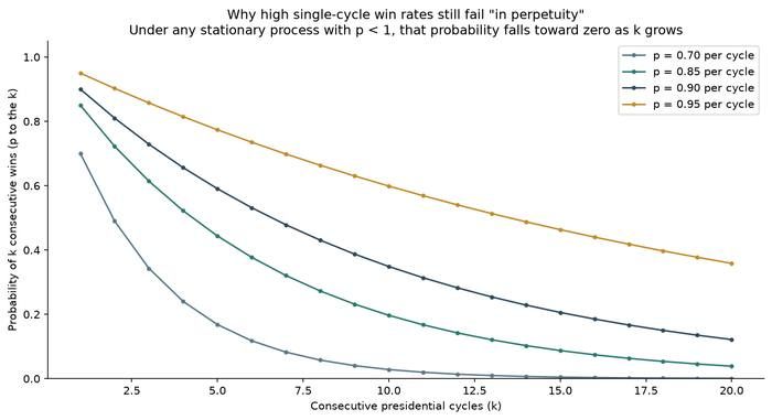
A single-election win probability, call it p, is not a permanence probability. If each presidential cycle is an independent draw with the same p, the chance of k consecutive wins is p to the k, and the expected length of a winning streak is 1 divided by (1 minus p) cycles. Those two formulas are enough to retire the word "perpetuity" as a mathematical claim.

At p equals 0.70, the expected streak is 3.3 cycles and ten straight wins have about a 2.8 percent chance. At p equals 0.85, the expected streak is 6.7 cycles and ten straight about 20 percent. At p equals 0.90 the expected streak is 10 cycles; at p equals 0.95, 20. Under any stationary process — one in which p itself does not change from cycle to cycle — p to the T goes to 0 as the horizon T goes to infinity. "In perpetuity" under fixed rules is not a large p; it is p equals 1. National shocks, mean reversion, and reapportionment reinforce that when election-process parameters stay fixed. What those formulas do not cover is the case in which winning itself changes the parameters of the next game — a non-stationary feedback loop taken up below.

§ 7The 2030 reapportionment twist

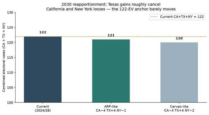
The weights themselves will change after the 2030 Census, in time for the 2032 and 2036 elections. Recent projections from Census Bureau estimates — including the American Redistricting Project, Carnegie Mellon apportionment research, and earlier Brennan Center work — converge on a striking pattern. Texas is widely projected to gain three to four electoral votes; California to lose three to four; New York to lose one or two. Under an ARP-style path of California minus 4, Texas plus 4, and New York minus 1, the combined CA+TX+NY total moves from 122 to 121. Under a Cervas-style path with New York minus 2, it moves to 120. Across the leading families, Texas's gains cancel the others' losses almost exactly, so the three-state anchor stays near 120 to 122. If they continue to vote as a bloc, the 35.6-versus-64.9 asymmetry survives the next reapportionment nearly intact.

§ 81962 Game Theory was based upon a different cultural reality

William H. Riker's The Theory of Political Coalitions, published in 1962, and the classical Hotelling–Downs model of spatial competition both assume a world that no longer matches today's institutional and cultural terrain. Riker's size principle says that in a zero-sum setting, competitors form coalitions only as large as they need to win, and that a permanently dominant-looking coalition is unstable because the losing side repositions toward equilibrium. Hotelling–Downs reaches a similar destination: when two competitors choose positions on a line, equilibrium collapses toward the median voter. Both frameworks treat election rules, turnout baselines, and the voter pool as fixed and roughly symmetric, and both assume voters fluidly cross coalition lines toward that median. Those were reasonable modeling choices in the civic, demographic, and media culture of the early 1960s. They are much harder to defend as complete descriptions of the system that has evolved since.

The California case shows the gap in structural terms. California's 54 electoral votes once sat inside competitive twentieth-century variance; the state swung regularly between coalitions. Once Coalition A consolidated statewide control, structural changes in the electorate and in the election process shifted California's baseline mean lean far beyond ordinary cycle-to-cycle noise. Coalition B's single-state win probability there has approached zero for multiple decades. That is not a temporary repositioning failure under fixed rules. It is a change in the parameters of the game itself — the state's mean lean and its variance — produced in part by who administers and designs the election process after winning it.

The same mechanism is why a CA+TX+NY lock can outrun 1962 theory. If Coalition A achieves statewide control in Texas and its 40 electoral votes, and then enacts election-process rules and turnout structures comparable to those that hardened California's baseline, Texas's mean lean and variance can shift the same way. The 40-vote block would then sit beside California's 54 and New York's 28 as an endogenous feedback loop: winning once alters the win probability p and the state lean of future contests. Static 1962 equilibrium models were never built to capture that loop. Under it, single-coalition dominance can stretch well beyond the five-to-seven consecutive terms that mark the longest twentieth-century streaks — roughly 1800–1824 at seven, 1860–1880 at six, and 1932–1948 at five, counted by election years alone. Those historical bounds describe more fluid voter pools and more symmetric institutional baselines. They are not a ceiling once the rules and the electorate themselves become prizes of winning.

§ 9What the mathematics actually says

Put the pieces together without rhetoric.

The Electoral College is a weighted voting game with quota 270 out of 538. Ten jurisdictions hold 254 of those votes. California, Texas, and New York together hold 122. When they align, Coalition A needs 35.6 percent of the remainder and Coalition B needs 64.9 percent. Exact Banzhaf and Shapley–Shubik indices show a modest large-state power premium, and the two-stage Penrose form still gives a California voter about 2.45 times a Wyoming voter's tipping power. The classic minimum-popular-vote bound sits near 22 percent of the national population. Correlated models show that moving Texas from a clear lean against A to a modest lean toward A lifts A's single-cycle win probability by roughly fifteen to twenty points. 2030 projections leave the combined CA+TX+NY weight almost unchanged.

Here is what all that math means in plain terms. With California, Texas, and New York locked together, Coalition A starts every race far ahead. Even after the 2030 Census moves some points from California and New York into Texas, those three still add up to about the same big block. If the rules stay still, pure chance says no winning streak lasts forever. But if Coalition A reshapes how voting works in Texas the way California changed, one side could stay on top far longer than old 1962 textbooks ever thought possible.